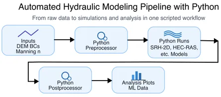
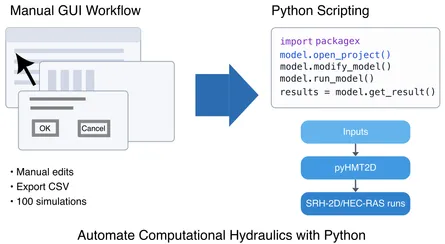
In Part 2 we used pyHMT2D to control HEC-RAS 2D and SRH-2D and convert results to VTK. In Part 3 we used the same machinery in a loop for automated calibration. Here we use it for Monte Carlo (MC) simulation: many runs with different parameter values (e.g., Manning’s $n$) to quantify uncertainty or build datasets for exceedance analysis, sensitivity, or machine learning.

Why Monte Carlo with pyHMT2D?

Uncertainty in inputs (roughness, inflow, geometry) propagates into uncertainty in outputs (water surface elevation, depth, velocity). Monte Carlo simulation repeatedly runs the model with parameters drawn from prescribed distributions. From the ensemble of results you can estimate exceedance probabilities, confidence intervals, or sensitivity indices. Doing this by hand is impractical—hundreds or thousands of runs, each with updated inputs and extracted outputs. With pyHMT2D, you script “for each sample: update parameters → run model → convert to VTK → extract quantities of interest” and optionally run cases in parallel.

If you haven’t done so yet, please read the Part 2 to understand how to install pyHMT2D and how it controls HEC-RAS 2D and SRH-2D from Python and converts their results to VTK.

Monte Carlo Examples in pyHMT2D

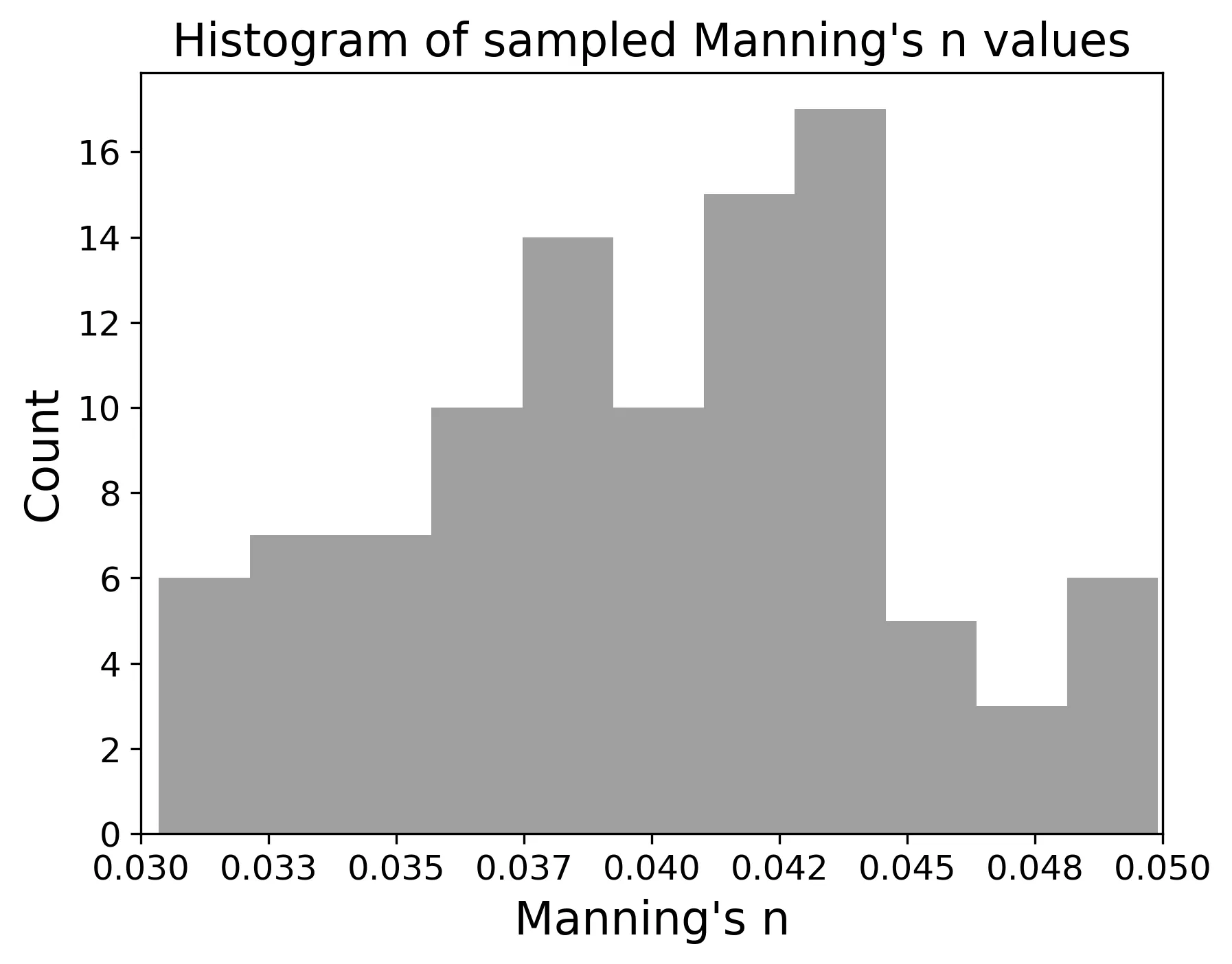
The pyHMT2D repository includes a Monte Carlo example under examples/Monte_Carlo/ that uses the Muncie 2D reach and varies Manning’s $n$ for the main channel according to a truncated normal distribution. The workflow has three stages: (1) generate parameter samples, (2) run the MC simulations with HEC-RAS 2D and/or SRH-2D, (3) convert and save each simulation result to VTK, (4) postprocess results (e.g., WSE exceedance probability at a monitoring point, and depth exceedance in the whole domain to VTK).

1. Generate parameter samples

A separate script generates Manning’s $n$ samples and writes them to a timestamped file:

• examples/Monte_Carlo/generate_parameters/generate_Monte_Carlo_parameters.py

It uses a truncated normal distribution (via scipy.stats.truncnorm) so that Manning’s $n$ for the main channel stays within a physical range (e.g., min/max) while having a chosen mean and standard deviation. The output file (e.g., sampledManningN_YYYY_MM_DD-HH_MM_SS.dat) is then copied into the model-specific folders so the same samples can be used for both HEC-RAS 2D and SRH-2D.

cd examples/Monte_Carlo/generate_parameters
python generate_Monte_Carlo_parameters.py
# Copy the generated parameter file into RAS_2D/Munice2D_ManningN_Monte_Carlo/ and SRH_2D/Munice2D_ManningN_Monte_Carlo/

The figure below shows the histogram of the sampled Manning’s $n$ values for the main channel with only 100 samples (to reduce the computation time). For real applications, you should generate more samples (e.g., 1000-10000) to get a more accurate distribution.

2. Run the Monte Carlo simulations

Each model engine (HEC-RAS 2D or SRH-2D) has a demo script that reads the parameter file, and for each Manning’s $n$ sample:

• Updates Manning’s $n$ in the model (pyHMT2D)
• Runs the 2D model (pyHMT2D controls the run as in Part 2)
• Converts results to VTK and extracts WSE at the monitoring point (pyHMT2D’s VTK/probing tools)

You can run in serial or parallel; the scripts use Python’s multiprocessing and a configurable number of processes (nProcess). For HEC-RAS, the plan should be set to use a single core so that multiple HEC-RAS instances can run in parallel without competing for cores.

• HEC-RAS 2D: examples/Monte_Carlo/RAS_2D/Munice2D_ManningN_Monte_Carlo/demo_HEC_RAS_Monte_Carlo.py
• SRH-2D: examples/Monte_Carlo/SRH_2D/Munice2D_ManningN_Monte_Carlo/demo_SRH_2D_Monte_Carlo.py

Example (after copying the parameter file into the folder):

cd examples/Monte_Carlo/RAS_2D/Munice2D_ManningN_Monte_Carlo
python demo_HEC_RAS_Monte_Carlo.py sampledManningN_YYYY_MM_DD-HH_MM_SS.dat

Each case is run in its own directory (e.g., under cases/); results are written to VTK. You can choose to delete case directories after each run to save disk space, since the VTK and extracted WSE are what matter for postprocessing.

3. Postprocess the results

The demos postprocess the ensemble to:

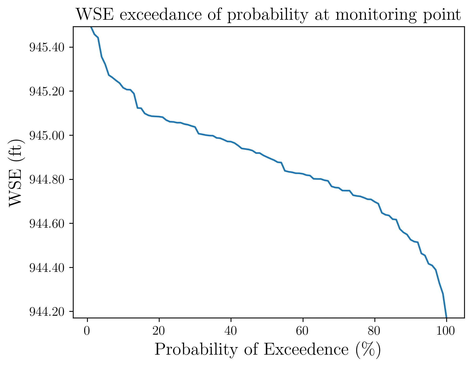
• WSE exceedance probability at the monitoring point: from final WSE at the monitoring point for every run, compute the empirical exceedance probability and plot it. The figure below illustrates this for the Muncie MC example.

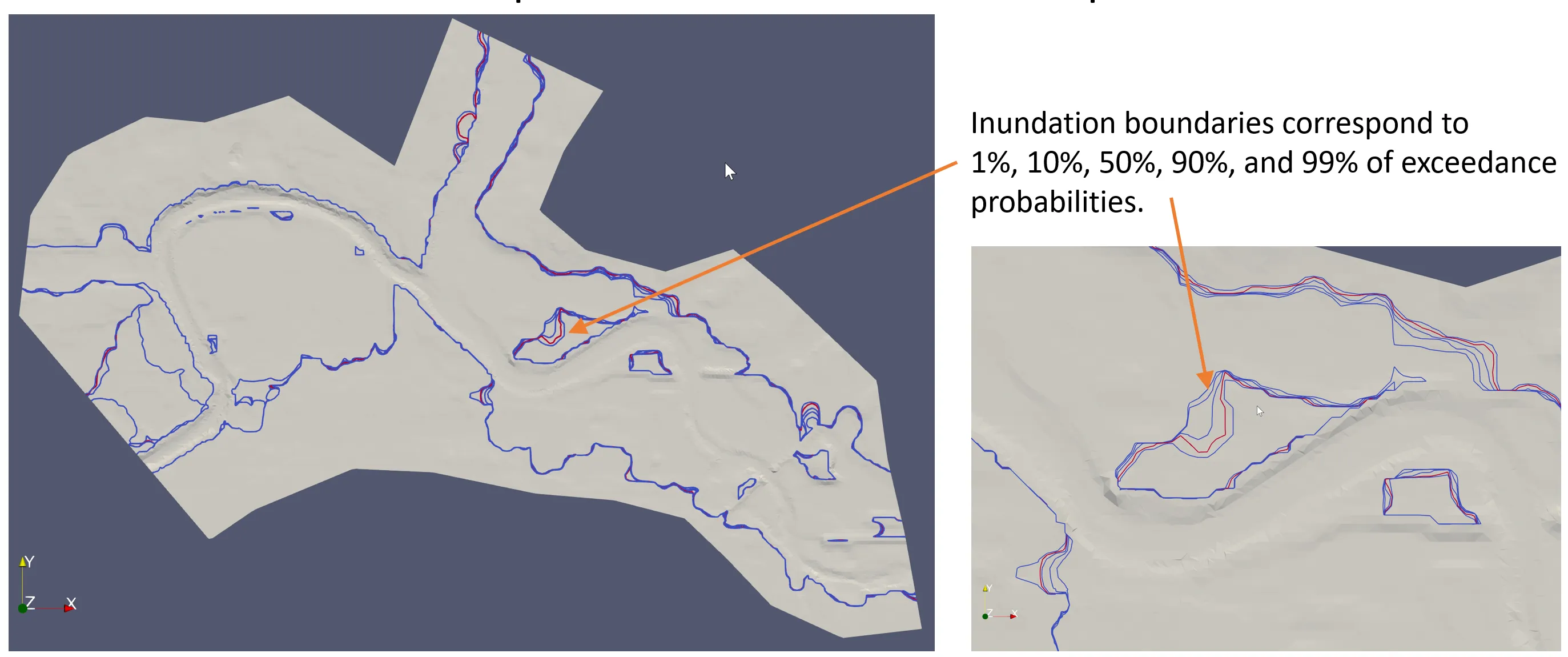
• Spatial exceedance of water depth: for each cell, compute the depth exceedance at selected percentiles (e.g., 99%, 90%, 50%, 10%, 1%) across the MC runs and write a single VTK file (e.g., water_depth_exceedance_of_probabilities.vtk) for visualization in ParaView. The figure below illustrates this for the Muncie MC example. The inundation boundaries are shown in different colors representing the 99%, 90%, 50%, 10%, and 1% probability of inundation, respectively.

So you get both point statistics (at the monitoring location) and field-level statistics (depth exceedance over the domain).

Serial vs parallel

The MC scripts can run in serial or parallel via a flag (e.g., bParallel) and a process count (nProcess). Parallel runs use multiprocessing on one machine; do not set nProcess higher than the number of available CPU cores. For HEC-RAS 2D, configure the plan to use one core so that multiple runs can proceed in parallel without oversubscribing.

Running the full workflow

1. Generate samples: From examples/Monte_Carlo/generate_parameters/, run python generate_Monte_Carlo_parameters.py, then copy the generated parameter file into both RAS_2D/Munice2D_ManningN_Monte_Carlo/ and SRH_2D/Munice2D_ManningN_Monte_Carlo/.
2. Run MC: From each of those directories, run python demo_HEC_RAS_Monte_Carlo.py <parameter_file> or python demo_SRH_2D_Monte_Carlo.py <parameter_file>.
3. Inspect outputs: Check the WSE exceedance plot and, if produced, the depth-exceedance VTK in the same folder. See the READMEs in each directory for more detail.

Summary

Monte Carlo with pyHMT2D reuses the same building blocks as in Part 2 and Part 3: model control, result conversion to VTK, and extraction of quantities (e.g., WSE at a point). The only addition is parameter sampling and batch execution (serial or parallel), plus postprocessing of the ensemble. Together, the four posts cover: (1) why automation matters, (2) pyHMT2D intro and run control + VTK, (3) automated calibration, and (4) Monte Carlo for uncertainty and exceedance analysis.

---

This is the fourth post in a series on automating computational hydraulics modeling. Read the previous post on calibration, or go back to the intro to pyHMT2D. Or go back to the index for the full series.