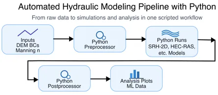
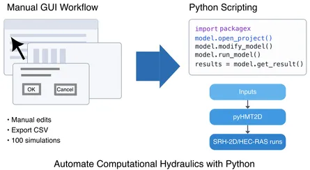
In the previous post, we saw how pyHMT2D controls HEC-RAS 2D and SRH-2D from Python and converts their results to VTK. Here we use that same machinery for automated calibration: finding Manning’s roughness coefficients that make simulated water surface elevations match observed high water marks (HWMs).

The Calibration Problem

You have a 2D model of a reach and a set of observed high water marks (HWMs)—measured or synthetic water surface elevations at specific locations. You want to choose model parameters (e.g., Manning’s $n$ for channel and floodplain) so that the simulated WSE at those points matches the observations as closely as possible. Doing this by hand—changing $n$, running the model, comparing, repeating—is slow and hard to reproduce. With pyHMT2D, you can wrap “run model → get WSE at HWM locations → compute misfit” in a single objective function and hand it to an optimizer. The optimizer then searches the parameter space automatically. The Python universe has many powerful optimizers. In the examples below, we use the Gaussian Process optimization (gp_minimize from scikit-optimize) to find the best-fit Manning’s $n$ values.

If you haven’t done so yet, please read the previous post to understand how to install pyHMT2D and how it controls HEC-RAS 2D and SRH-2D from Python and converts their results to VTK.

Muncie 2D Calibration Examples in pyHMT2D

The pyHMT2D repo includes two calibration examples that share the same setup:

• examples/calibration/RAS-2D/Munice2D_ManningN_calibration
• examples/calibration/SRH-2D/Munice2D_ManningN_calibration

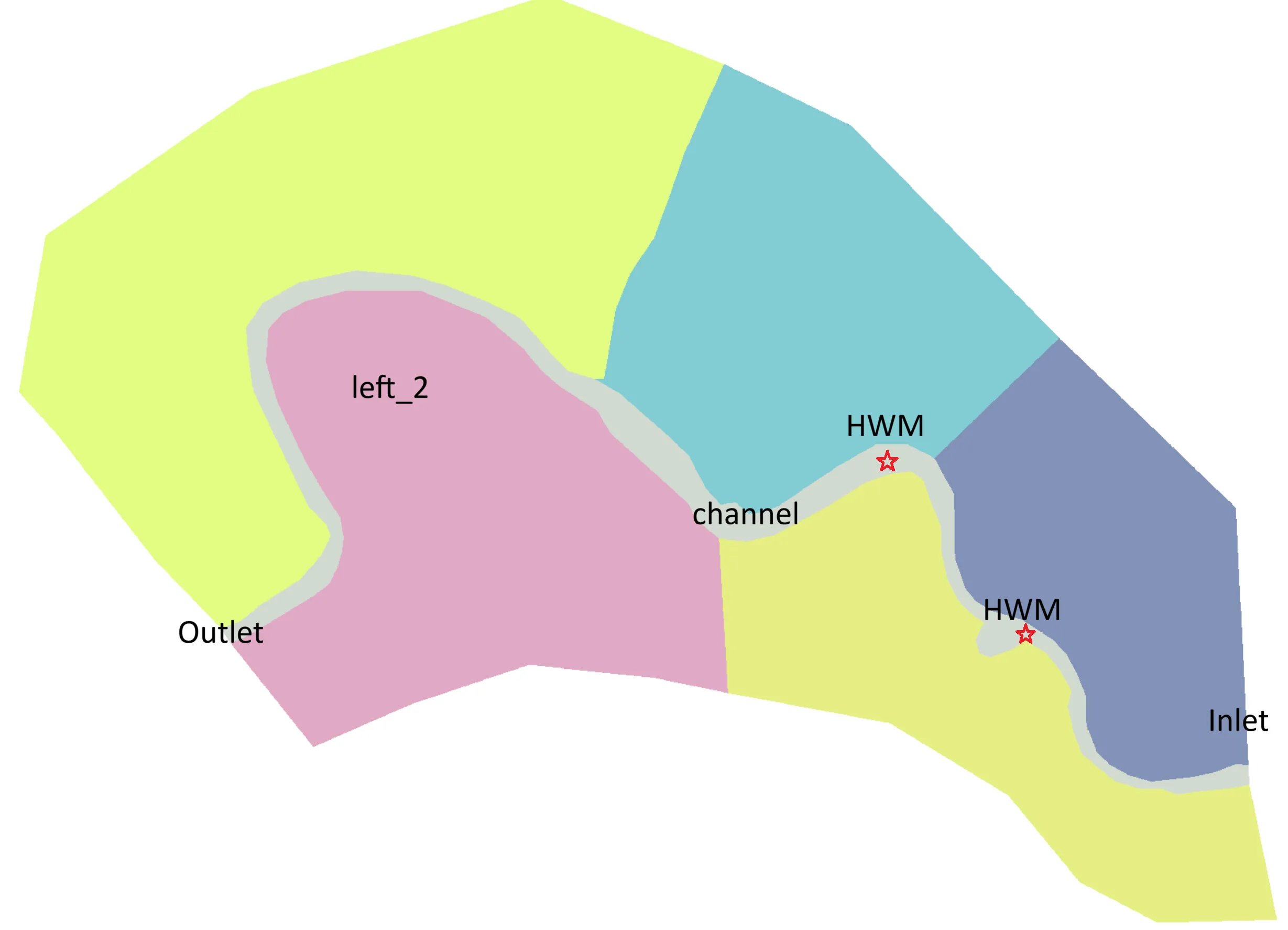
Both use the Muncie 2D reach. There are two Manning’s $n$ parameters to calibrate: one for the main channel and one for the floodplain (left_2). The “observations” are synthetically generated from the same Muncie case with known $n$ values (0.04 for the channel and 0.06 for the floodplain), so we can check whether the optimizer recovers them.

The figure below shows the case layout and the two HWM locations.

Calibration Workflow

In both examples the workflow is:

1. Define the objective: Misfit between simulated and observed WSE at all HWM points (e.g., RMSE).
2. Set parameter bounds: Manning’s $n$ for channel and floodplain within a reasonable range, e.g., [0.02, 0.08].
3. Run an optimizer (e.g., gp_minimize from scikit-optimize):
   • For each candidate $(n_{\text{channel}},n_{\text{floodplain}})$:
     • Update Manning’s $n$ in the model input (using pyHMT2D).
     • Run the 2D model (pyHMT2D controls the run as in Part 2).
     • Convert results to VTK and probe WSE at the HWM coordinates (pyHMT2D’s VTK/probing tools).
     • Compute the objective (e.g., RMSE) and return it to the optimizer.
   • The optimizer proposes the next parameter set until a computational budget (e.g., 50 evaluations) is exhausted.
4. Save and visualize: Record the calibration trajectory and, optionally, run a final case with the best parameters.

I will not give an in-depth explanation of “how pyHMT2D runs the model” or “how VTK conversion works”; that is exactly what we covered in the previous post. Calibration simply loops over that workflow and feeds the misfit into an optimization routine.

HEC-RAS 2D Example

The RAS-2D calibration is driven by:

• examples/calibration/RAS-2D/Munice2D_ManningN_calibration/demo_calibration_RAS_2D.py

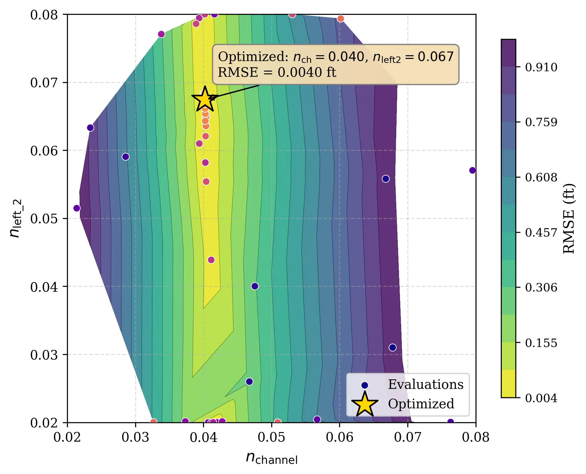
The script uses pyHMT2D’s HEC_RAS_Model and RAS_2D_Data to update Manning’s $n$ in the geometry, run HEC-RAS, convert results to VTK, and probe WSE at the HWM points. The objective is minimized with Gaussian Process optimization (gp_minimize from scikit-optimize). After tens of function evaluations, the optimizer typically finds values close to the true values of 0.04 and 0.06 for the channel and floodplain, respectively.

The figure below shows a typical calibration trajectory: sampled $(n_{\text{channel}},n_{\text{floodplain}})$ and the objective (contour). The search concentrates where the misfit is low. It is also interesting to see the objective function landscape. It is clear that the objective function is more sensitive to the main channel and less so to the floodplain (left_2). This makes physical sense because the flow resistance in the main channel has more direct impact on the backwater effect.

SRH-2D Example

The SRH-2D counterpart is:

• examples/calibration/SRH-2D/Munice2D_ManningN_calibration/demo_calibration_SRH_2D_gp.py

The idea is the same: pyHMT2D updates Manning’s $n$ in the SRH-2D input, runs the model, converts to VTK, and probes WSE at the HWMs. The same type of GP-based optimizer (e.g., gp_minimize) is used. You get a similar calibration trajectory and a set of best-fit Manning’s $n$ values. Both examples use the same Muncie geometry and synthetic HWMs, you can compare calibrated $n$ and WSE between HEC-RAS 2D and SRH-2D. However, don’t expect both calibrations to find the same best-fit Manning’s $n$ values because the two models are not exactly the same.

Running the Examples

From the pyHMT2D clone (with the package installed in development mode):

• RAS-2D: cd examples/calibration/RAS-2D/Munice2D_ManningN_calibration then python demo_calibration_RAS_2D.py
• SRH-2D: cd examples/calibration/SRH-2D/Munice2D_ManningN_calibration then python demo_calibration_SRH_2D_gp.py

Ensure HEC-RAS and/or SRH-2D (e.g., via SMS) are installed and that paths in the scripts match your system. For more detail, see the READMEs in each calibration folder.

What’s Next?

Automated calibration is one way to use pyHMT2D’s run control and result extraction in a loop. Another is Monte Carlo simulation: many runs with different parameters (e.g., inflow or roughness) to explore uncertainty or build datasets for sensitivity analysis. In the next post, we’ll look at Monte Carlo with pyHMT2D.

---

This is the third post in a series on automating computational hydraulics modeling. Read the previous post for an introduction to pyHMT2D and run control, or continue to the next post for Monte Carlo simulation. Or go back to the index for the full series.